Google Summer of Code 2022: DigiKam Image Quality Sorter Algorithms Improvement
Project description
The main idea of IQS in digiKam is to determine the quality of an image and convert it into a score. This score is based on four factors sabotaging image: blur, noise, exposure, and compression. The current approach helps determine whether images are distorted for one of these reasons. However, the current algorithm also presents some drawbacks: It demands lots of fine-tuning from the user’s side and cannot work on the aesthetic image. So, I propose the solution of the deep learning algorithm. While the dataset and the paper for aesthetic image quality assessment are free to use, we are capable of constructing a mathematical model that can learn the pattern of a dataset, hence, predicting the score of quality. As deep learning is an end-to-end solution, it doesn’t require the setting for the hyperparameter. Therefore, we can reduce most of the fine-tuning parts to make this feature easier to use
Check out the IQS Proposal for more info about the description and algorithm of the project.
First week 13/06/2022 - 19/06/2022
As described in the proposal, the first week is dedicated to experimenting and reproducing the result of two target algorithms NIMA and musiq.
I aim to test and train the deep learning model following the algorithms. Hence, only the code needed for these tasks is extracted from their repos. All is published in my own repose iqs digikam.
These are my principal task in my first week :
- Install environment for running python code of NIMA and musiq.
- Download dataset of EVA and AVA datasets.
- Write training and testing script for NIMA.
- Adapt the label of 2 datasets for the context of NIMA.
Achievement in the first week :
- For now, I can train, evaluate and predict each image using python.
- Using the pre-trained model of the paper achieves a good performance: MSE = 0.3107 (means the variance is 3.1 on the scale score of IQS digiKam)
Current problem:
- Most images are labeled with a score of around 5. This is reasonable as if the annotator can not be sure about the quality of the image, they will give a score of 4, 5, or 6. It creates the problem of evaluating the model. The metric MSE will show that it is a accepted model even when the model will predict all the images with a score of 5. These two images show the distribution of the score on 2 datasets: AVA and EVA:
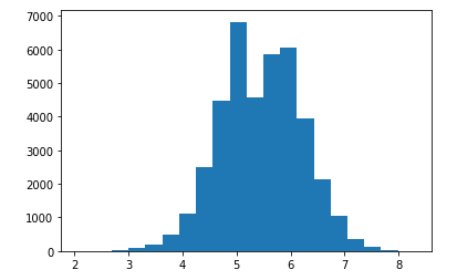
Figure1 : distribution of score of AVA dataset
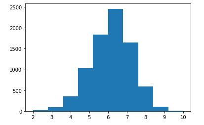
Figure2 : distribution of score of EVA dataset
Ideal to resolve:
- Augment data of different ranges / reduce data of concentrated range to have a balance dataset
- Change metric that considers more weighted on the result of different region score
Second week 20/06/2022 - 26/06/2022
As described in the last post, the current metric for regression (MSE) is not suitable for imbalanced data. Hence, I consider a branch new metric :
- As our use-case at the end is the classification between 3 classes: rejected, pending, and accepted image, hence, I split the data into three classes with the same meaning. As most of the images are in class pending, the data is still imbalanced. Hence, I use F1 score for evaluation.
- Spearman’s rank correlation coefficient is a metric to evaluate the similarity between 2 distributions. Hence, the more similar between prediction and reference, the better the performance of the model
After having these two metrics, I re-evaluate the function model of NIMA: The checkpoint given by the paper still achieves the best performance: 0.589 on the F1 score for the class of digiKam.
As I explained last week, we need a balanced dataset that the score is evenly distributed. I did research on a new dataset for image quality assessment:
- SPAQ dataset is a dataset for image quality assessment that evaluates each image by a score from 0 to 100.
For the sake of achieving the performance of the paper without using the checkout proposed by the image, I fine-tune the model for various situations:
- Fine-tuning on number of epochs: number of training-dense epochs and number of full training models. The best combination is three epochs for dense training and seven for full model training.
- Testing on base model variant: MobileNet, InceptionV2, InceptionV3, VGG16. The model using VGG16 showed the best precision.
- However, I did not yet archive the performance as the paper.
Upcoming task:
- Combining various datasets could create a balanced dataset.
- Training on the combined dataset
- Training from the pre-trained weight of the paper.
Third week 27/06/2022
Although the research wasn’t finished, we can already use the pre-trained model published by NIMA with acceptable performance. Hence, following the timeline in my proposal, the next step would be using the model in C++.
Before integrating into digiKam’s repo, I tried to compile a small C++ with OpenCV. Then, using module DNN of OpenCV to read the image, read the pre-trained model, and calculate the score of the image. To do that, there are some steps to do:
- On the Python side, the pre-trained model file must be freeze the weight. This is a specific technique so the model file could be read by OpenCV
- On the C++ side, having OpenCV from 4.5.5 is a requirement.
- At last, we only need to read the model from the file, read the image, and calculate the model’s output. This is a small example of inference
Fourth and Fifth week 04/07/2022 - 17/07/2022
As mentioned in the second week, I changed the metric to consider the problem as classification with three classes. However, changing the metric doesn’t help us improve the model’s performance. Because the model still trains with the loss function of the regression problem. Secondly, training data is still imbalanced as their score is always around 5. The work of these two weeks is to resolve the imbalanced dataset problem. I have come to a reasonable solution for digiKam.
In fact, in the end, we would like to have a label of rejected, pending, or accepted for an image. So this is a classification problem. That’s why I realize these steps :
- Re-label the dataset by only three classes. I separate classes by it a quality score.
- To have a balanced dataset, I use only 9000 images for each class, as most of the images are in a pending dataset.
- Change the last layer of the model to dense softmax. This is a layer using softmax activation function. Hence, the result is the percentage of an image belonging to each class.
- Change the lost function applied to train the model, from earth movers distance to categorical entropy.
- Change also the metric to evaluate the model: the first is the percentage of true prediction on the evaluation set; the second is the f1 score on each dataset. While the first matrix is more natural to human understanding, the second represents the model’s capacity to recognize each class.
After experimenting, the model shows the expected result. I use the evaluation set of AVA after labeling with classification to evaluate the model. There are 14.702 images with 3.626 images from class 2 ( accepted images), 6.862 images from class 1 ( pending images), 4.214 images from class 1 ( rejected images). The percentage of true prediction is 0.721. F1 score is 0.764 0.674 0.741 on each class. This file shows the label and the prediction of each image of the AVA dataset.
These results after training and testing with different base model and hyperparameter. I conclude to this configuration :
- Base model : InceptionResNetV2
- Batch size : 16
- Learning rate : 0.0005
- Number epochs : 8
- dropout rate : 0.75
Main current problem : As the purpose is to have balanced data, I choose the threshold as 5 and 6, which means if the score <= 5, the image is labeled as rejected, 5 < score <= 6 is for pending, and the rest is for a accepted image. This is too objective, so the images labeled 0 are not really bad, or the images labeled two are not too well, which confuses the model.
solutionSolution Using a combined dataset could be a good solution.
Sixth week 18/07/2022 - 24/07/2022
As I would like to spend more time on research after the first evaluation, I changed a little in my plan. This week, I realized the main classes of aesthetic detection and integrated into digiKam. As I have changed the model’s architecture in the last week, the aesthetic detection cli should also be changed. The main problem is performing the preprocessed image from python to c++.
Before implementing the core class of aesthetic detection, I did a small unit test. I get three images that are classified as a accepted image in the AVA dataset and three images of rejected quality that are already in the data of image quality sort.
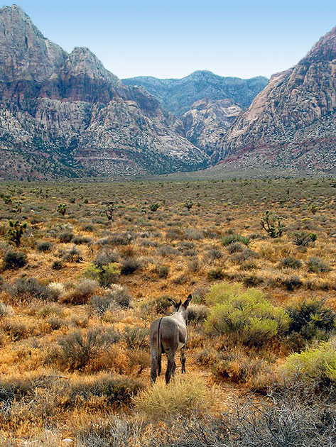
Figure3: Aesthetic image from the AVA dataset
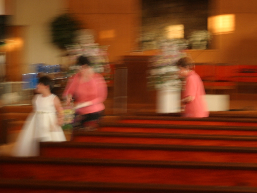
Figure4: Rejected image from IQS digiKam unit test
After the unit test, I implement the aesthetic detector to pass the unit test. Fortunately, the architecture of the detector of image quality sorter is well defined. Hence, I implement only the main functions of aesthetic detection based on the aesthetic cli. There are only three main methods :
- Preprocessing: The preprocessing process should be the same to what is done in python. The image is transformed from blue-green-red mode to red-green-blue mode, then resized to 22x224 with INTER_NEAREST_EXACT interpolation. In the end, each pixel is normalized to -1 and 1.
- Serving model: The model is loaded from a PB file. This is the model file of TensorFlow. Opencv dnn is developed well in this path.
- Postprocessing: The output of a deep learning model is only a matrix with the score. Based on the meaning of the last layer, these scores have a different meanings. In our case, the score is a matrix of 3 float numbers representing the probability that the image belongs to each class.
The implementation of aesthetic detection passes all unit tests. However, we have the problem of the similarity between aesthetic cli and aesthetic detector. While they give the exact class prediction, the score is slightly different. The reason is the way they read the image from the file. While the cli uses imread method from OpenCV to read the picture, the detector uses a loading image thread of digikam with the size of 1024 x 1024. This could cause the problem in the future.
Current problem: The file model path should be dynamic to the repo of digikam. However, the file is too large and can not be handled by Github. For now, I hardcoded the link to the model file. The model file can be downloaded from here
First phase resume
This part is dedicated to resuming the achievements, problems, TODO list, and ideas in the first phase of GSOC22. Achievements:
- (research side) Complete data pipeline for AVA and EVA dataset.
- (research side) Analyze data to retrieve the main problem: an imbalanced dataset -> most images are labeled with a score from 4 to 6 on a scale of 10.
- (research side) Train, test, and experiment NIMA on AVA and EVA dataset -> confirm the problem of an imbalanced dataset.
- (research side) Change the problem to 3-classes classification based on digikam context, re-implement data labeling and change the last layer of the model to adapt to the new context. Achieve an acceptable result on the AVA dataset evaluation set: 72.1% of accurate prediction.
- (integration side) Implement aesthetic detection cli that can receive a model path and an image path to get the image’s quality score.
- (integration side) Implement aesthetic detector classes in digikam code base and aesthetic unit test.
Problem:
- (research side) Labeling class images based on their score is too objective. Hence, the model easily confuses between rejected and pending photos or pending and accepted images.
- (research side) MUSISQ is not yet well researched as it is implemented in the non-popular framework JAX, and OpenCV can not read the pre-trained file.
- (integration side) The position of the model file should be managed dynamically by the repo.
TODO:
- (research side) Concatenate dataset and train on this dataset -> more generalized dataset better model
- (research side) Research on Musiq.
- (integration side) Implement UI of aesthetic detection and management of model file.
Seventh week 25/07/2022 - 31/07/2022
As explained in the resume of last week, we can improve the model by combining different datasets. The main idea is to create a most generalized dataset. These experiments help us evaluate better the performance of the model’s architecture. At first, we need to choose which dataset to be combined. AVA and EVA dataset is a good choice as all of their images are aesthetic. On the other hand, the dataset Koniq10k contains images with different levels of distortion. Although images with distortion are not necessarily aesthetic, images that are too distorted are terrible. Hence, I added rejected photos of Koniq10k to the evaluation set.
These are some hyper-parameters for the combined dataset:
- Dataset AVA : rejected images ( score <= 5); pending images ( score <= 6); accepted images ( score > 6)
- Dataset EVA : rejected images ( score <= 5); pending images ( score <= 7); accepted images ( score > 7)
- Dataset Koniq10k: get only rejected image with a score < 40.
After having the evaluation set, I re-evaluated the model that was produced in the first phase. As expected, I observed a significant loss of accuracy on the combined evaluation set. In the same way as concatenating datasets, I created the combined dataset for training. These are some portions of each class in the evaluation set and training set :
| Data set | % of rejected image | % of pending image | % of accepted image |
|---|---|---|---|
| Evaluation set | 27.56% | 44.99% | 27.50% |
| Training set | 29,65% | 35.48% | 34.87% |
After experimenting and fine-tuning with the same process in the first phase, I achieved a significant improvement
| The model | Accuracy on AVA | Accuracy on combined dataset |
|---|---|---|
| Model trained on AVA dataset | 0.721 | 0.542 |
| Model trained on combined dataset | 0.70 | 0.64 |
TODO: In the next week, I would like to improve the model by changing the architecture inside. The main idea is to use a smaller base model but dense of fully connected at the end of the model.
Eighth week 01/08/2022 - 07/08/2022
In this week, I would like to optimize the performance of the model in 2 directions : inference time and accuracy. To optimize accuracy, I perform some experiments including : increase the batch size of training, increase the size of image for training, and insert a fully-connected after the last layers of the model.
As I used the InceptionNet as the base model, there are always a layer of batch normalization. This layer need a large batch size to achieve the generalization because the distribution of the batch will be closer to the real population. From batch size 16, I experiment with batch size 32 and 64. The following figure shows the improvement.
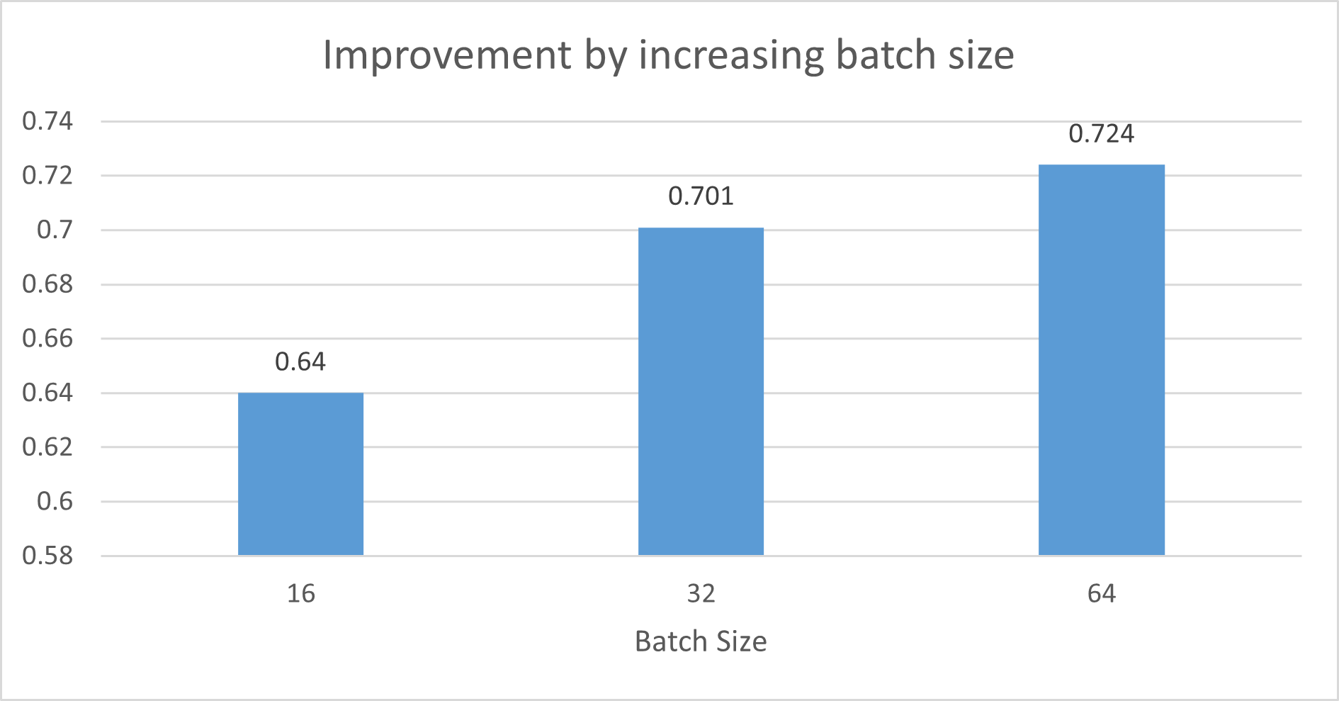
Figure5 : Improvement by increasing batch size
Secondly, I increase the image size at the input of the model. There are two reasons. At first, we can extract more information in bigger image. Hence, in theory, the model can be more accurate. However, we can not use too large image because as it would be a huge burden on Ram. Secondly, the origin design of InceptionNet receive the image with size 299x299. Actually, we use the input size as 224x224 as we want to use the pre-trained weights of ImageNet. The following figure shows the improvement of increasing image size. However, I can not use whatever the image size because of the limitation of my computational resource. A vary large image size make me to decrease the batch size, hence, we loose the benefit of the last idea.
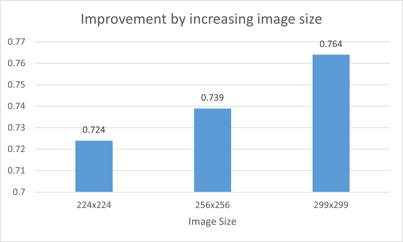
Figure6 : Improvement by increasing image size
In the other hand, I would like to minimize the inference time. It is important to calculate faster in digiKam. Hence, I replace the base model InceptionResNetV2 by InceptionV3. I decrease the number of parameter from 55.9M to 23.9M. This change reduces also the accuracy of the model. Hence, I inserted a fully-connected dense before the last layer. I calculate also the inference time on one image using CPU. The following table indicates the difference model I used.
| The model | Accuracy on combined dataset |
|---|---|
| Base model : InceptionResNetV2 | 0.764 |
| Base model : InceptionV3 | 0.752 |
| Base model : InceptionV3 + Dense FC | 0.783 |
Ninth week 07/08/2022 - 14/08/2022
The main task of this week is implementation the user interface (UI) for aesthetic image detector. When using this feature, the user doesn’t need to config different parameter. Hence, this interface of configuration is likely the next figure.
After testing the feature on digikam, I observe that the calculation is quite slow. The reason is that for each image, the model will be loaded from the file to Ram. We can optimize this process by loading the model only one time at the beginning of the feature.
In this week, I made also a research on Vision transformer(Vit) which is the main idea behind the algorithm musiq. The Vision Transformer, or ViT, is a model for image classification that employs a Transformer-like architecture over patches of the image. An image is split into fixed-size patches, each of them are then linearly embedded, position embeddings are added, and the resulting sequence of vectors is fed to a standard Transformer encoder. In order to perform classification, the standard approach of adding an extra learnable “classification token” to the sequence is used.
The motivation of this approach is to find the relation between different part of image, then, find the important region of image that effect most on the quality. This is in fact the used case of aesthetic image. For example, image with blurred background have only a part that is sharped. Hence, this part is the most important to classify the quality of the image.
The algorithm musiq uses the same idea. However, I do not use directly the code of musiq because of 2 reasons. At first, the model is coded in the new framework JAX. This is the new framework of google for implementing deep learning model. However, it is unstable. It poses a lots of bugs and unexpected error to reproduce the result. Secondly, the model file from JAX is not supported yet by the library DNN of opencv. So, using directly their code can not conclude a useble model for digiKam. The structure of musiq is much large. Hence, I implement only the main idea : Vision Transformer.
The architecture of my model is presented in the following figure.
The result is quite disappointed. Although the model is smaller than NIMA, the complexity is too high. The complexity of the Transformer is quadratic (O(n^2 × d)) with n is the number of patch and d is the complexity to process on a patch. In our case, with n is 16 (image is separated by 4 rows and 4 columns), the calculation is 128 times bigger than calculation for a patch. For each path, their is a correspondent residual net. The consequence of high complexity is the slowness in training and evaluation. In further, because of the limitation of my GPU, I can not train the model with a high batch size. Hence, the result is not impressive.
| The model | Accuracy on combined dataset |
|---|---|
| InceptionV3 + Dense FC | 0.783 |
| Vision Transformer | 0.547 |
Tenth week 15/08/2022 - 21/08/2022
In this week, I focus on realizing the model. In the experiment of seventh week, I have 2 observations:
- At first, adding new dataset makes the model more generalized. The evidence is that the metric on both old dataset and the new ones increase. The reason for this phenomenon is that, instead of adapting only one distribution of on dataset, the model is forced to learn a more generalized distribution.
- Secondly, although all of our training dataset are for image quality assessment, their subjective is extremely different. EVA and AVA contains only artistic images. In fact, most of images has similar quality. Koniq10k contains natural images that score by the level of distortion. Hence, image with blur or noise or overexposure is labeled rejected images.
By these observations, I re-arrange the data for training. Images from dataset like AVA or EVA are labeled for standard image or accepted image. While image from distorted dataset like Koniq10k is labeled as rejected image or standard image. Hence, we make an assumption for definition of aesthetic image : rejected image is the normal image with distortion; pending image is the normal image without distortion or artistic image but badly captured; accepted image is a good artistic image.
In addition, I found the dataset SPAQ. It contains normal dataset captured by smartphone. The images in SPAQ with score <= 60 are extremely distorted. Hence, I labeled these images as rejected image.
To evaluate the idea, I calculate not only the accuracy on combined evaluation set, but also the accuracy on each class of each component dataset. The following table shows the result :
| Dataset | Accuracy |
|---|---|
| Combined dataset | 0.783 |
| AVA | 0.812 |
| EVA | 0.751 |
| Koniq10k | 0.743 |
| SPAQ | 0.974 |
This model will be used in digiKam
Eleventh week 15/08/2022 - 21/08/2022
In this week, I focus on 2 tasks :
- Until now, we load the model one time for each image. Hence, it consumes a lot of time, and it is not propriate for our case. We should load the model only one time for each we call the feature.
- After having aesthetic detector with the right model, I evaluate its performance compared to Image Quality Sorter by distortion. I evaluate on 2 features : calculation time and capacity to recognize aesthetic image.
The first task is accomplished by using the static property of C++. I add a static member of model and 2 static methods to load and unload model in AestheticDetector.
In the second task, I run Image Quality Sorter in two ways : distortion detection ( using 4 distortion detector ) and aesthetic detection. To compare calculation time, I run two ways on 5000 images. While the distortion detection takes 14 minutes and 23 seconds to finish the task, the aesthetic detector takes only 8 minutes. To evaluate the capacity of aesthetic detector, I run two ways on EVA dataset. In this test, I would like to verify the capacity of aesthetic detector compared to using 4 distortion detector. The result is impressive. While distortion detection achieves 38.91% for accuracy of the class, aesthetic detection achieves 83.09%
| Metric | distortion detection | aesthetic detection |
|---|---|---|
| Running time on 5000 images | 863 seconds | 527 seconds |
| Accuracy on EVA dataset | 38.91% | 83.09% |
Final phase resume
This part is dedicated to resuming the achievements and problems in the last phase of GSOC22. Achievements:
- (research side) Add Koniq10k and SPAQ dataset for training and evaluation.
- (research side) Define the property of image for each classes :
- Rejected image is the normal image with distortion
- Pending image is the normal image without distortion or artistic image but badly captured
- Accepted image is a good artistic image.
- (research side) Fine tune model structure to maximize the metric and minimize calculation time
- (research side) Make a first try on Vision Transformer, the original idea of Musiq.
- (integration side) Implement UI for aesthetic detection.
- (integration side) Improve the aesthetic detection’s performance by caching the model for run time of IQS.
- (integration side) Evaluate the advantage of IQS using distortion detection and using aesthetic detection.
Problems:
- (research side) Although the algorithm Musiq reports a better performance than NIMA, I still can not reproduce its result.
- (research side) Most of images for training are natural image. Hence, there are very little people their. Hence. the model could be fail to predict on people image.